|
|
Geometry & Linear AlgebraLines in the plane and Least squares method - A uniqueness problem |
A very compact form to express a system of linear equations
\[
\left\{
\begin{array}{rcrcrcrcr}
a_{11}x_1 &+& a_{12}x_2 &+& \cdots &+& a_{1n}x_n &=& b_1 \\
a_{21}x_1 &+& a_{22}x_2 &+& \cdots &+& a_{2n}x_n &=& b_2 \\
&\vdots & & & & & & \\
a_{m1}x_1 &+& a_{m2}x_2 &+& \cdots &+& a_{mn}x_n &=& b_m
\end{array}
\right.
\]
is to use matrix language adopted from Linear Algebra.
We introduce the
coefficient matrix
\( A = (a_{ij})_{m{\times}n} \), the column vector
\( \mathbf{b}\) for the right side known numbers and the column \( \mathbf{x}\) for the unknowns.
Then the system looks like
\[
\left(
\begin{array}{cccc}
a_{11} & a_{12} & \cdots & a_{1n} \\
a_{21} & a_{22} & \cdots & a_{2n} \\
\vdots & \vdots & \ddots & \vdots \\
a_{m1} & a_{m2} & \cdots & a_{mn}
\end{array}
\right)
\left(
\begin{array}{c}
x_1 \\
x_2 \\
\vdots \\
x_n
\end{array}
\right)
=
\left(
\begin{array}{c}
b_1 \\
b_2 \\
\vdots
\\ b_m
\end{array}
\right)
\]
and briefly
\[
A\mathbf{x} = \mathbf{b}.
\]
Example 1. Solve
\[
\left\{ \begin{array}{rcrcr}
x_1 &+& x_2 &=& 3 \\
-2x_1 &+& 3x_2 &=& 1 \\
2x_1 &-& x_2 &=& 2 \end{array} \right.
\]
Solution. There is no solution. However there might be some convenient answer, ''compromise''.
Let \( A \) be the coefficient matrix.
Then the normal equation has the form
\[
\begin{array}{crcl}
& A^TA \mathbf{x} &=& A^T \mathbf{b}\\[3pt]
\iff & \left( \begin{array}{rrr} 1 & -2 & 2 \\ 1 & 3 & -1 \end{array} \right)
\left( \begin{array}{rr} 1 & 1 \\ -2 & 3 \\ 2 & -1 \end{array} \right)
\left( \begin{array}{c} x_1 \\ x_2 \end{array} \right)
&=& \left( \begin{array}{rrr} 1 & -2 & 2 \\ 1 & 3 & -1 \end{array} \right)
\left( \begin{array}{r} 3 \\ 1 \\ 2 \end{array} \right) \\[5pt]
\iff&
\left( \begin{array}{rr} 9 & -7 \\ -7 & 11\end{array} \right)
\left( \begin{array}{c} x_1 \\ x_2 \end{array} \right)
&=& \left( \begin{array}{r} 5 \\ 4 \end{array} \right) \\[5pt]
\iff&
\left( \begin{array}{c} x_1 \\ x_2 \end{array} \right)
&=& \left( \begin{array}{c} \frac{83}{50} \\ \frac{71}{50} \end{array} \right)
\end{array}
\]
The Least squares solution to \( A\mathbf{x} = \mathbf{b} \) is
\[
\widehat{\left( \begin{array}{c} x_1 \\ x_2 \end{array} \right)}
= \left( \begin{array}{c} \frac{83}{50} \\[3pt] \frac{71}{50} \end{array} \right)
= \left( \begin{array}{c} 1{,}66 \\[3pt] 1{,}42 \end{array} \right)
\]
Unfortunately, it turns out that if we use a different representation of the lines, we get different solutions!
Example 2. For example, if we take \[ \left\{ \begin{array}{rcrcr} 10x_1 &+& 10x_2 &=& 30 \\ -2x_1 &+& 3x_2 &=& 1 \\ 2x_1 &-& x_2 &=& 2 \end{array} \right. \] we have exactly the same plane lines, but the Least Squares solution would be \[ \widehat{\left( \begin{array}{c} x_1 \\ x_2 \end{array} \right)} = \left( \begin{array}{c} \frac{691}{427} \\[3pt] \frac{1181}{854} \end{array} \right) = \left( \begin{array}{c} 1{,}62 \\[3pt] 1{,}38 \end{array} \right) \] Problem. What is the least squares solution for the previous system, when the first equation is multiplied by \( 0 \)? Answer: \[ \widehat{\left( \begin{array}{c} x_1 \\ x_2 \end{array} \right)} = \left( \begin{array}{c} \frac{7}{4} \\[3pt] \frac{6}{4} \end{array} \right) = \left( \begin{array}{c} 1{,}75 \\[3pt] 1{,}50 \end{array} \right) \]
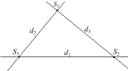
Dynamical figures (''Sketches'') allow us to experiment the problem in a visual way!The geometric representations of the linear equations \[ a_{i1} x_1 + a_{i2} x_2 = b_i \] are lines in the plane. Remember that a system of such equations can be written in linear algebra language as matrix equation \[ A\mathbf{x} = \mathbf{b}, \] where \( \mathbf{x} \) is the vector of the unknowns \( x_i \).
|
|
In this dynamic Sketch you can make parallel moves for the lines by dragging with the computer mouse the
points \( P_1 \), \( Q_1 \) and \( R_1 \).
The point \( \widehat{\mathbf{x}} \) is the Least squares solution of the equations on the screen.
Problems1. Explain why \( \widehat{\mathbf{x}} \) is moving, though the lines do not move when you change \( k_1 \), \( k_2 \) or \( k_3 \) (push Scale equations first).
2. How is \( \widehat{\mathbf{x}} \) moving when you vary \( k_1 \) from negative to positive direction?
3. What is the curve drawn by \( \widehat{\mathbf{x}} \) when \( P_2 \) is moving around circle and all other given points are fixed? |
|
|
Puzzle 1 ProblemTry to find the least squares solution \( \widehat{\mathbf{x}} \) of the system of the equations for the lines in the Sketch.Give the coordinates of \( \widehat{\mathbf{x}} \): |
|
|
Puzzle 2 ProblemTry to find the least squares solution \( \widehat{\mathbf{x}} \) of the system of the equations for the lines in the Sketch.Give the coordinates of \( \widehat{\mathbf{x}} \): |
|
|
Puzzle 3 ProblemTry to find the least squares solution \( \widehat{\mathbf{x}} \) of the system of the equations for the lines in the Sketch.Give the coordinates of \( \widehat{\mathbf{x}} \): |
|
|
Puzzle 4 ProblemHere you can move one of the lines by dragging the points \( P_1 \) and \( P_2 \). Try to find such equations for the first line so that the Least squares solution \( \widehat{\mathbf{x}} \) is the given black point \( \widehat{\mathbf{x}}' \). Give your equations: Are there many different solutions? |
|
|
Puzzle 5 ProblemHere you can move two of the lines by dragging the points \( P_1 \), \( P_2 \), \( Q_1 \) and \( Q_2 \). Try to find such positions for the lines that the Least squares solution \( \widehat{\mathbf{x}} \) is the given black point \( \widehat{\mathbf{x}}' \). Are there many different solutions? |
|
|
Puzzle 6 ProblemHere you can move all the lines. Try to find such positions for the lines that - the Least Squares Solution \( \widehat{\mathbf{x}} \) is the given black point \( \widehat{\mathbf{x}}' \) and - turning lines does not make the solution move. Are there many different solutions? What can you say about this (or these) solutions? |
|
|
In this Sketch you can make parallel moves for the lines by dragging with the computer mouse the
points
\( P_1 \),
\( Q_1 \),
\( R_1 \) and
\( S_1 \).
You can turn the lines around with the points
\( P_2 \),
\( Q_2 \),
\( R_2 \) and
\( S_2 \).
Also you can multiply the equations by numbers \( k_1 \), \( k_2 \), \( k_3 \) and \( k_4 \). Try all the buttons in the Sketch. ProblemDescribe all possible positions of \( \widehat{\mathbf{x}} \) for the 4 given lines when \( k_1 \), \( k_2 \), \( k_3 \) and \( k_4 \) belong to \( \mathbb{R} \). |
|
|
We define \[ A = \left( \begin{array}{cc} k_1 a_1 & k_1 b_1 \\ k_2 a_2 & k_2 b_2 \\ k_3 a_3 & k_3 b_3 \end{array} \right), \quad \mathbf{x} = \left( \begin{array}{c} x_1 \\ x_2 \end{array} \right), \quad \mathbf{c} = \left( \begin{array}{c} k_1 c_1 \\ k_2 c_2 \\ k_3 c_3 \end{array} \right), \quad \] The matrix equation \( A\mathbf{x} = \mathbf{c} \) has in general no solution. The least squares solution \( \widehat{\mathbf{x}} \) of the normal equation \[ A^T\! A \mathbf{x} = A^T \mathbf{c} \] is such that \[ F(\mathbf{x}) = F(x_1,x_2) = || A \mathbf{x} - \mathbf{c}||^2 = (\mathbf{x}^T\,A^T - \mathbf{c}^T)(A\mathbf{x} - \mathbf{c}) \] is minimum for \( \mathbf{x} = \widehat{\mathbf{x}} \). We denote by \( d(\mathbf{x},L) \) the distance from the point \( \mathbf{x} \) to line \( L \). Computing \( F(\mathbf{x}) \) we get: \[ F(\mathbf{x}) = k_1^2 \left(d(\mathbf{x},d_1)\right)^2 + k_2^2 \left(d(\mathbf{x},d_2)\right)^2 + k_3^2 \left(d(\mathbf{x},d_3)\right)^2 \]
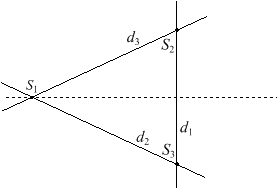
1. If the triangle defined by the lines \( d_1 \), \( d_2 \) and \( d_3 \) is isosceles (let us say \( S_1 S_2 = S_1 S_3 \)), on what line do you expect to find \( \widehat{\mathbf{x}} \) (see Figure 2) ?
|
|
2. If the triangle is equilateral where is \( \widehat{\mathbf{x}} \)?
3. The distances of \( \widehat{\mathbf{x}} \) to the sides of the triangle are proportional to the lengths of the corresponding sides to a certain power \( r \): \[ \frac {d(\widehat{\mathbf{x}},d_1)}{{l_1}^r} = \frac {d(\widehat{\mathbf{x}},d_2)}{{l_2}^r} = \frac {d(\widehat{\mathbf{x}},d_3)}{{l_3}^r} \] Guess what is the value of \( r \)?
Note: If \( r = -1 \), the point \( \widehat{\mathbf{x}} \) would be the center of gravity; if \( r = 0 \), the point \( \widehat{\mathbf{x}} \) would be the center of the inner circle.
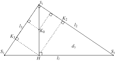
4. If the triangle is rectangular, e.g. \( d_2 \perp d_3 \), on what line do you find \( \widehat{\mathbf{x}} \) (see Figure 3)?
|
|
\[ \frac {H K_2}{S_1 S_3} = \frac {H K_3}{S_2 S_1} \ \textrm{since the triangles are similar} \]
|
|
You can move the lines by dragging the intersections \( A \), \( B \) and \( C \).
With the Sketch control button you can see step by step: - the point \( C_1 \) and the line parallel with line \( CA \) at distance \( |AC| \) |
|
|
You can move the lines by dragging the intersections \( A \), \( B \) and \( C \).
With the Sketch control button you can show and hide the three steps: - the point \( A_2 \) and the line parallel with line \( AB \) at distance \( |AB| \) |
|
|
You can move the lines by dragging the intersections \( A \), \( B \) and \( C \).
With the Sketch control button you can show and hide the three steps: - the point \( A_3 \) and the line parallel to line \( CA \) at distance \( |CA| \) |
|
|
You can move the lines by dragging the intersections \( A \), \( B \) and \( C \).
Here you can see the intersection of the first two lines and then check whether also the third will fit. |
|
|
You can move the lines by dragging the intersections \( A \), \( B \) and \( C \).
On the left side you can see how the symmedian ray of the median \( AA_m \) from \( A \) is constructed, reflecting over the bisector. On the right side you see a quick image of the previous construction from the point \( A \). ProblemsThe intersection of \( BC \) with \( A\widehat{\mathbf{x}} \) (or \( A O_1 \)) is denoted by \( P \).1. Show that \( b^2 |PB| = c^2 |PC| \), where \( b = |CA| \) and \( c = |AB| \). 2. Show that \( AP \) is a symmedian of the triangle \( ABC \), that is, the image of the median in the reflection along the inner bisector shown on the picture. 3. Are the three symmedians of a triangle concurrent? |