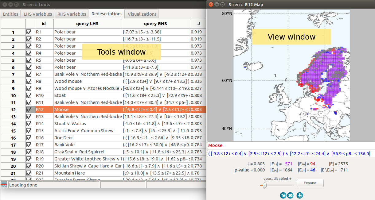
The Tools window is unique, it is the main siren window. It contains several tabs.
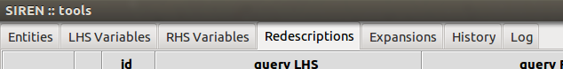
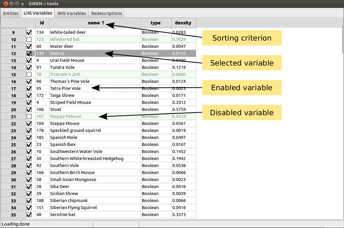
Two tabs contain lists of variables.
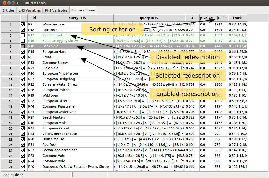
Three tabs contain lists of redescriptions.
Finally,
Tabs can be shown or hidden via the interface menu .
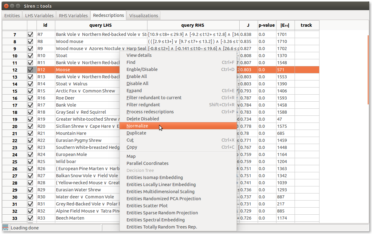
The main means to manipulate variables or redescriptions, depending on which tab you are currently viewing, are available via the Edit menu and the contextual menu opened by right click.
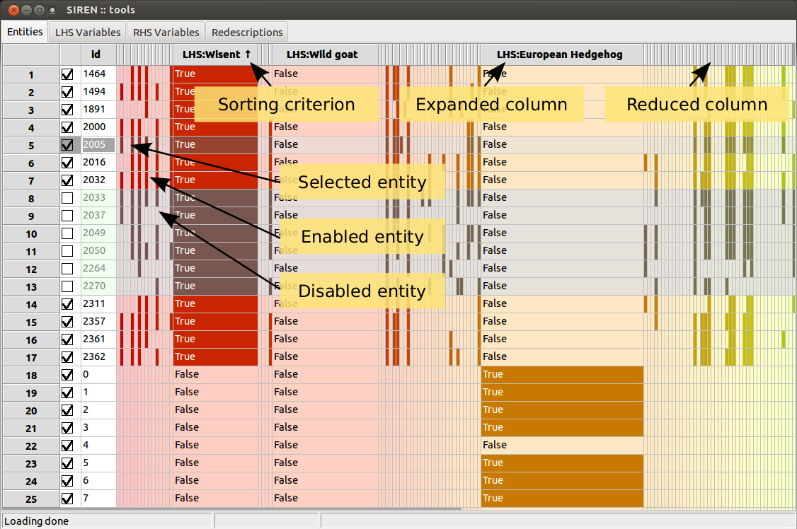
List items can be enabled/disabled by checking/unchecking the corresponding box in the left column. All items in a list can be enabled/disabled simultaneously. Lists can be sorted based on the value of the different fields displayed by clicking on the column header.
Redescriptions can be cut, copied, and pasted from and to different positions in the lists and from one list to the other and vice-versa. All disabled redescriptions can be deleted at once.
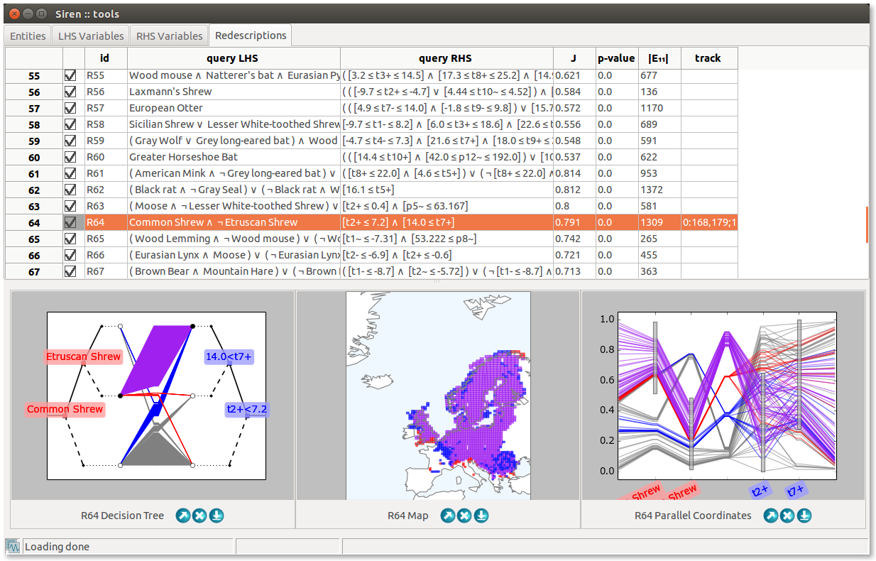
A view window allows to visualize a redescription, to edit it and launch mining and expansion. Several views of different types of the same redescription can be opened simultaneously. They are linked together an to the original redescription in the list so that edits and selections made in one view are reflected in the list and other views.
A View window can be opened with a double click on a variable or redescription in a list from the Tools window.

Both queries can be edited using the text boxes. If the syntax of a query is incorrect, Siren will not be able to parse it and it will fall back on the previous correct query.
Queries are parsed when ENTER is pressed, in order to avoid parsing error due to partial edits.
Redescriptions statistics are shown below the queries.
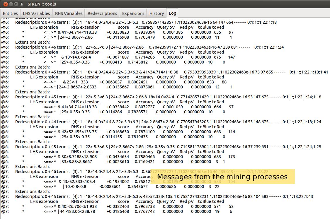
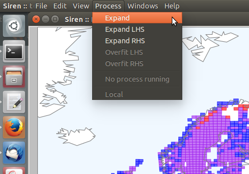
Expansion can be started by pressing the Expand button. The expansion will be delegated to a background process. It can be interrupted via the menu , where running task are listed. Redescriptions generated during the expansion will be appended to the list of redescriptions in the Expansions tab.
Clicking on the entities, represented as lines or dots, highlights them accross the different views for the redescription with labels showing the entities’s ID to allow identifying them. It is also possible to enable highlighting and labeling the entities on hover (by activating Hover entities in the Interface preferences), and jumping to the entity in the entities list on click (by toggling ).
Some actions are visualization-specific. A slider allows to set the opacity of disabled entities in all visualizations except the tree diagrams. For parallel coordinates plots, another slider allows to adjust the level of details by limiting the fraction of entities drawn.
In case of projections, setting controls allow to set parameters and the data can be projected anew by clicking the Reproject button.
A polygon drawing tool allows to select groups of contiguous areas.
In tree diagrams, clicking on a leaf allows to add and remove the corresponding branch to the query.
Then, Simplify LHS and Simplify RHS buttons allow to simplify the diagrams of the tree associated to the left-hand side and right-hand side queries, respectively.
In parallel coordinates plots, the range of literals can be adjusted interactively by dragging the corresponding grey boxes.
Plotting the visualizations to separate windows is one possibility. In such a case, all controls and stats are available, as shown above.
An alternative is to plot the visualization to a grid inside a dedicated tab of the main window. In that case, to accomodate more visualizations, controls are not shown, but the queries and stats are still visible.
An entry of the Edit menu allows to choose whether visualizations should be plotted by default into new separate windows or inside the visualization tab.
The plots can be popped out of the tab into separate windows, and vice-versa using the arrow buttons. The cross allows to close the view. Rows and columns can be added and dropped from the visualization grid by clicking on the green bars to the bottom and to the right of the grid, and the red bars to the top and to the left of the grid respectively. On deletion of a row or column of the grid, all views it contains are closed. The grid cell where the next visualization will be plotted is highlighted, a free cell can be chosen by simply clicking on it. If no free cell is available, the next plot will replace the oldest views in the grid, effectively deleting it.
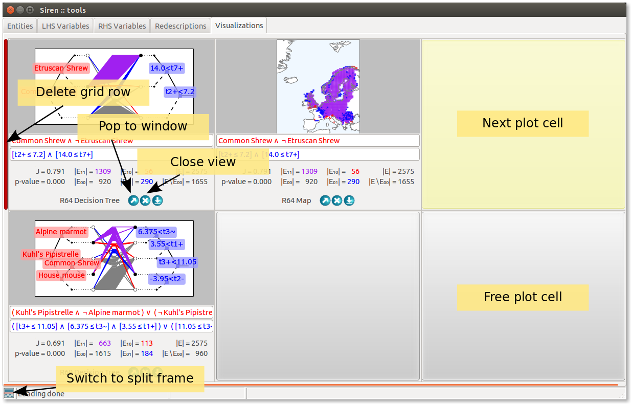
Finally, clicking on the colored button on the bottom-left corner of the main window allows to split the main window horizontally into two frames, so as to show the grid of visualization beneath a list, for instance the list of redescriptions. To save further space the stats and queries are not shown in that case. Clicking anew on the colored button restores the main window to a single frame.
Note
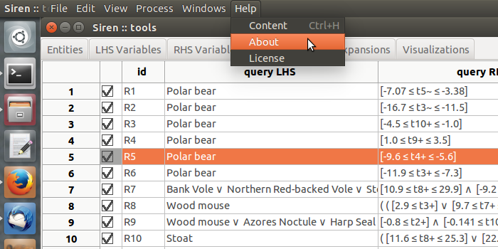
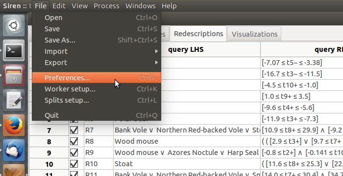
The main menu of Siren is at the top of the Tools window.
Here is a summary of functionalities available throught the menu.
The File submenu provides import, export, opening and saving functionalities and setting the preferences.
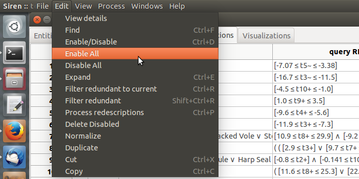
The content of the Edit submenu depends on the tab or view currently active.
If the tab contains redescriptions, it will also allow to filter the redescription and to copy, cut and paste them.

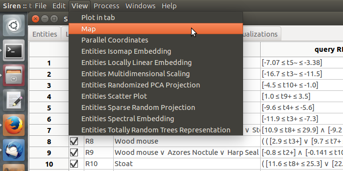
If the tab contains redescriptions or variables the View menu will allow to open a view window to visualize the selected item. Possible visualizations for an item might differ. For instance, if a redescription cannot be represented as a tree, the tree diagram entry of the menu will be disabled, the normalize function should be applied first.
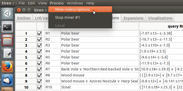
The Process menu allows to start mining redescriptions and contains a list of running task and allows to interrupt any of them.
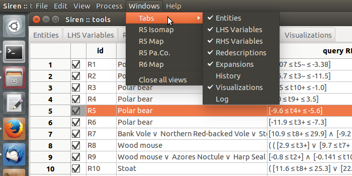
The Windows menu contains a list of tabs and allows to show or hide any of them.
It also contains a list of Views currently opened sorted by redescription, allowing to access any of them and close all at once.
Many Edit and Views functionalities can also be accessed via the contextual menu upon right-click on a redescription.
Note
Siren provide means to send computations to an external server, thereby helping to maintain the responsiveness of the interface
In addition, to help study how well the redescriptions mined using a particular set of parameters generalize to unseen entities, Siren allows to easily partition the data, run the algorithm on a selected subset of the data and compare accuracy and support of the results.
To pass mining and projection computation on to an external server, the settings for communicating with that server can be set in the Worker setup... in the File menu. This allows to set the IP address (set to local to disable the client-server mode), port and authentication key, and to test the connection and check whether some processes are already being run on the server.
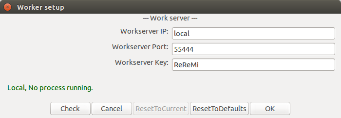
Of course, the mining server should be setup with the relevant settings using the provided server_siren.py script.
Running the following, for instance, initializes a server on the feedback-loop listening on port 55444 with authentication key atk and having 4 workers (i.e. handling at most 4 different delegated tasks simultaneously).
python server_siren.py 127.0.0.1 --portnum=55444 --authkey=atk --max_k=4
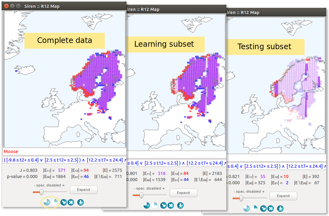
Finally, Siren also allows to partition the data to study how redescription characteristics vary on different data subsets.
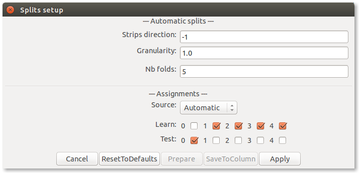
The settings for doing this can be accessed through the Splits setup... in the File menu.
The upper half of the dialogue box allows to choose parameters to generate a data partition automatically, by selecting a column or coordinate to whose values will direct the partition. A value greater than zero identifies a data column by its position, while a value lower than zero indentifies a coordinate, a value of zero means that the data will be partitioned randomly. That is, 1 corresponds to the first column on the left-hand side, while 12 corresponds to second column on the right-hand side assuming the left-hand side contains 10 columns, and -1 corresponds to the first coordinates dimension, i.e. the longitudes. The granularity allows to tune the width of the bands, while the number of folds defines the number of partitions returned.
The lower half of the dialogue box allows to choose the source, either desactivating the splits, using the automatic settings described above to generate partitions or extracting it from a data column (a categorical variable, where each category will generate a partition). Once this is set, the partitions can be generated. Next, the resulting partitions can be assigned to the learn (L) or test (T) folds. A partition can be stored in the data by encoding it as an additional column, so that it can be loaded again later on.
After the splits setup as been applied, new columns will appear in the redescription lists, showing the statistics (accuracy, p-Values, support) on the learn and test folds.
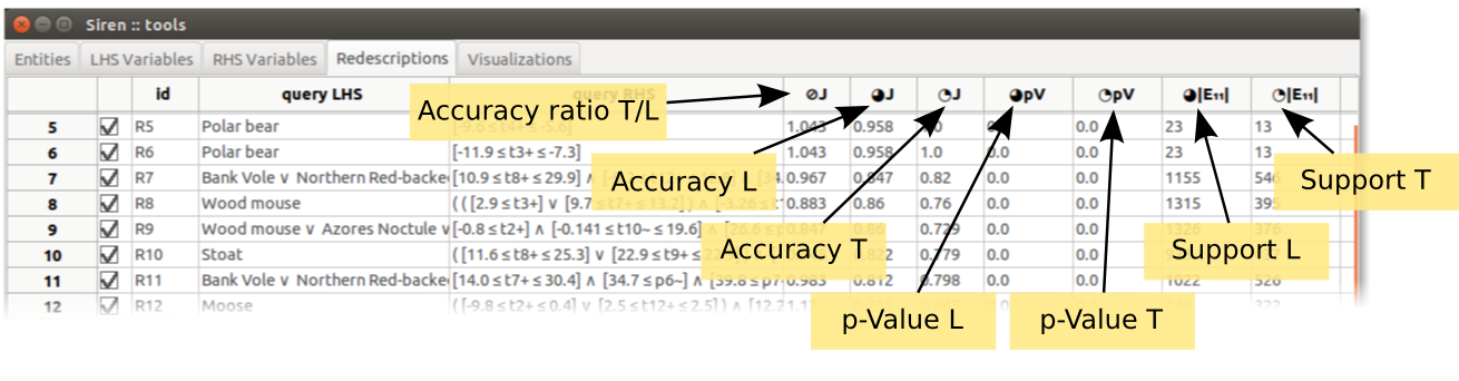
In views, a pair of buttons will appear allowing to focus on the complete data or on either split.